Code
ewf_standings <- readr::read_csv(
  "https://raw.githubusercontent.com/probjects/ewf-database/main/data/ewf_standings.csv"
)Get ready to kick off your analysis and celebrate the remarkable achievements in women’s football! 🥳🥇⚽️
This week’s TidyTuesday dataset dealt with the Women’s English Football League performances between 2011-2023.⚽️
More details on this dataset here 👈
The source of the data and the code used to obtain Figure 1 is delineated through Section 2.1 to Section 2.4.
ewf_standings <- readr::read_csv(
"https://raw.githubusercontent.com/probjects/ewf-database/main/data/ewf_standings.csv"
)library(tidyverse)
library(stringr)
library(glue)
library(ggrepel)
library(ggplot2)
library(ggtext)
library(sysfonts)
library(showtext)
# caption handles
swd <- str_glue("#SWDchallenge: June 2024 • Source: Synthetic data from ChatGPT<br>")
li <- str_glue("<span style='font-family:fa6-brands'></span>")
gh <- str_glue("<span style='font-family:fa6-brands'></span>")
mn <- str_glue("<span style='font-family:fa6-brands'></span>")
# plot colors
bkg_col <- colorspace::lighten("#e3d5eb", 0.05)
title_col <- "#3d3d3d"
subtitle_col <- "#3d3d3d"
caption_col <- "#72647D"
text_col <- colorspace::darken("gray40" , 0.2)
# fonts
font_add('fa6-brands','fontawesome/otfs/Font Awesome 6 Brands-Regular-400.otf')
font_add_google("DM Serif Display", regular.wt = 400, family = "title")
font_add_google("Urbanist", regular.wt = 400, family = "subtitle")
font_add_google("Quattrocento Sans", regular.wt = 400, family = "text")
font_add_google("Merriweather", regular.wt = 400,family = "caption")
showtext_auto(enable = TRUE)
X_icon <- glue("<span style='font-family:fa6-brands'></span>")
caption_text <- str_glue("{li} Arindam Baruah | {X_icon} @wizsights | {gh} arinbaruah | Source: TidyTuesday |#rstudio #ggplot2")
theme_set(theme_minimal(base_size = 15, base_family = "text"))
# Theme updates
theme_update(
plot.title.position = "plot",
plot.caption.position = "plot",
legend.position = 'plot',
plot.margin = margin(t = 10, r = 15, b = 0, l = 15),
plot.background = element_rect(fill = bkg_col, color = bkg_col),
panel.background = element_rect(fill = bkg_col, color = bkg_col),
axis.title.x = element_text(margin = margin(10, 0, 0, 0), size = rel(1), color = text_col, family = 'text', face = 'bold'),
axis.title.y = element_text(margin = margin(0, 10, 0, 0), size = rel(1), color = text_col, family = 'text', face = 'bold'),
axis.text = element_text(size = 10, color = text_col, family = 'text',face = "bold"),
panel.grid.minor.y = element_blank(),
panel.grid.major.y = element_line(linetype = "dotted", linewidth = 0.1, color = 'gray40'),
panel.grid.minor.x = element_blank(),
panel.grid.major.x = element_blank(),
axis.line.x = element_line(color = "#d7d7d8", linewidth = .2),
)ewf_standings <- ewf_standings %>% mutate(Status = case_when(position == 1 ~ "Champions",
season_outcome == "Relegated to tier 2" ~ "Relegations",
.default = "All other teams"))# Ensure ggplot2 and ggrepel are loaded
library(ggplot2)
library(ggrepel)
title_text <- "How do the goals scored and conceded vary for \n those at the top and bottom of the table in Women's EFL?"
subtitle_text <- "<span style='color: #496250;'>Analyzing the number of goals scored and conceded by each participating Women’s English Football Club between 2011 and 2023 reveals a compelling picture of <br> contrasting performances in front of the goal. Championship-winning teams consistently demonstrated strong defenses, <strong> with none conceding more than 20 goals <br> in a season </strong>. However, the number of goals scored by these champions varied widely, ranging from 20 to 100 goals. This suggests that a <strong> solid defense is a more <br> significant contributor to championship success than a high-scoring offense </span>.</strong>
<span style='color: darkred;'>Conversely, for clubs relegated to lower divisions, <strong> none scored more than 25 goals in a season </strong>, while the number of goals conceded ranged from 20 to 75.<br> This indicates that for teams at the bottom of the table, offensive struggles are more detrimental than defensive issues. In summary, as we move lower in the <br> standings, <strong> offensive performance becomes increasingly critical compared to defensive solidity.</span> </strong>"
note_text <- "Most dominant champion"
# Create the plot
pl <- ggplot(data = ewf_standings, aes(x = goals_for, y = goals_against, text = team_name)) +
geom_point(aes(color = Status), size = 1) + geom_point(
data = filter(ewf_standings, Status == "Relegations"),
aes(color = Status),
size = 4
) +
geom_point(
data = filter(ewf_standings, Status == "Champions"),
aes(color = Status),
size = 4
) +
geom_text_repel(
data = filter(ewf_standings, Status == "Relegations"),
aes(label = team_name),
size = rel(5),
nudge_x = -10,
nudge_y = 20,
fontface = "bold"
) +
geom_text_repel(
data = filter(ewf_standings, Status == "Champions"),
aes(label = team_name),
size = rel(5),
# nudge_x = 7,
#nudge_y = -15,
fontface = "bold"
) +
geom_richtext(
aes(
x = 75, y = 62,
label = note_text,
family = "text"
),
vjust = 1.1,
label.color = NA,
size = rel(9),
fill = bkg_col
) +
geom_curve(
aes(x = 75, xend = 96, y = 50, yend = 12),
curvature = 0.2,
arrow = arrow(length = unit(0.15, "cm"), type = "closed"),
color = "black"
) +
scale_color_manual(values = c("Champions" = "gold", "Relegations" = "darkred","All other teams" = "gray"),
name = "Season outcome") +
labs(caption = caption_text,
x = "Goals scored",
y = "Goals conceded",
title = title_text,
subtitle = subtitle_text) +
theme(legend.position = "top",
legend.title.position = "top",
legend.title = element_text(
color = text_col,
hjust = 0.5,
family = "text",
face = "bold",
size = rel(2.5),
),
legend.text = element_text(
color = text_col,
family = "text",
size = rel(2),
face = "bold"
),
plot.title = element_text(
size = rel(4),
family = "title",
face = "bold",
color = title_col,
lineheight = 0.3,
margin = margin(t = 5, b = 5),
hjust = 0.5
),
plot.subtitle = element_markdown(
size = rel(2),
family = 'subtitle',
color = subtitle_col,
hjust = 0,
lineheight = 0.2,
margin = margin(t = 5, b = 1)
),
plot.caption = element_markdown(
size = rel(1.5),
family = 'caption',
color = caption_col,
lineheight = 0.3,
hjust = 0.5,
halign = 0,
margin = margin(t = 10, b = 10)
),
axis.title = element_markdown(
size = rel(2.5)
),
axis.text = element_markdown(
size = rel(2.5)
)
)
ggsave("EWF_standings.png",pl,dpi = 300,height = 6, width = 10)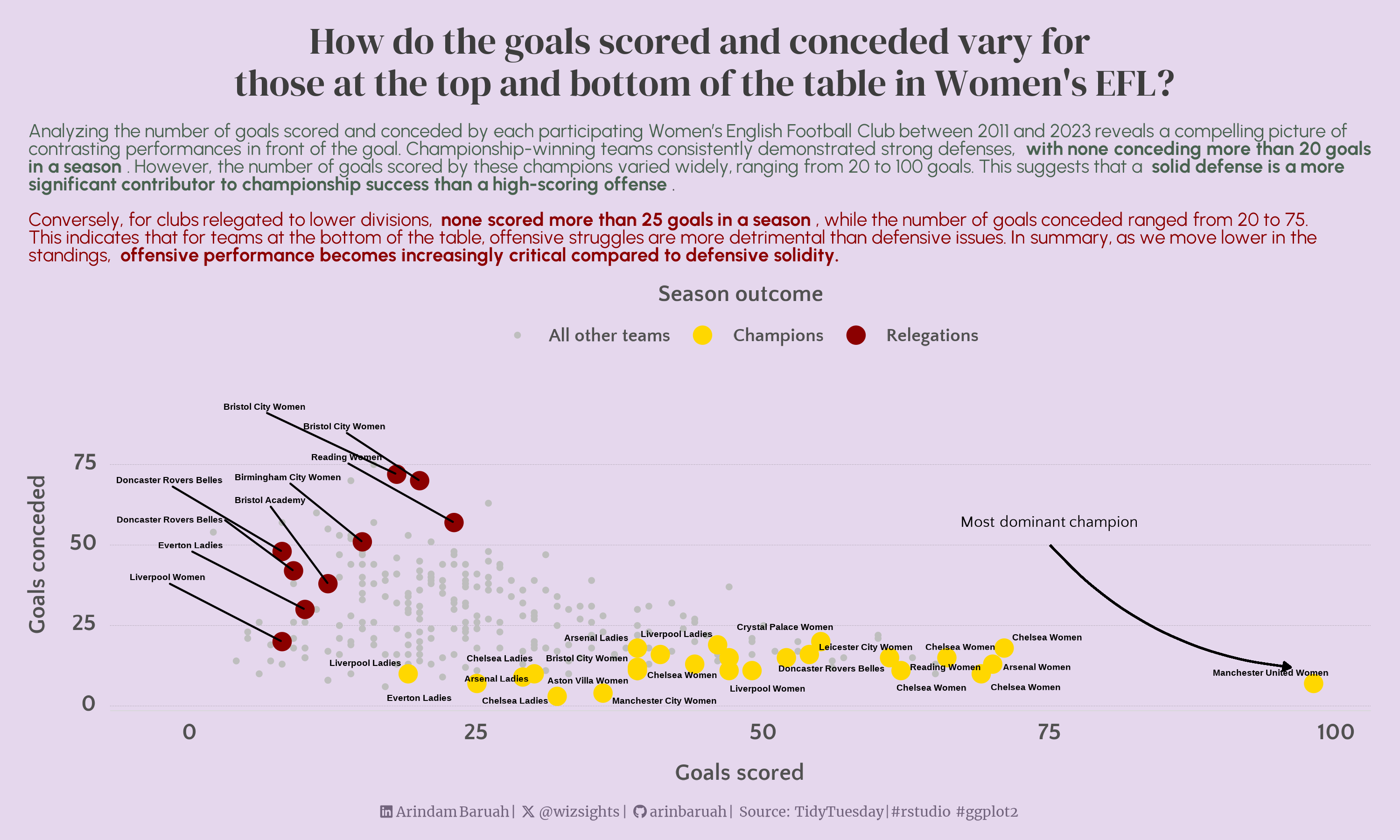
Figure 1 illustrates the variation in the number of goals scored and conceded for Women’s EFL Champions and Relegations. For the current analysis, league performances between the seasons of 2011 to 2023 were ocnsidered.
So what do we learn from this ? 🤔🕵🏻♀️
Key insights based on 2011-2023 standings👇
tidyverse: Wickham H, Averick M, Bryan J, Chang W, McGowan LD, François R, Grolemund G, Hayes A, Henry L, Hester J, Kuhn M, Pedersen TL, Miller E, Bache SM, Müller K, Ooms J, Robinson D, Seidel DP, Spinu V, Takahashi K, Vaughan D, Wilke C, Woo K, Yutani H (2019). “Welcome to the tidyverse.” Journal of Open Source Software, 4(43), 1686. doi:10.21105/joss.01686 https://doi.org/10.21105/joss.01686.
glue: Hester J, Bryan J (2024). glue: Interpreted String Literals. R package version 1.7.0, https://CRAN.R-project.org/package=glue.
ggrepel: Slowikowski K (2024). ggrepel: Automatically Position Non-Overlapping Text Labels with ‘ggplot2’. R package version 0.9.5, https://CRAN.R-project.org/package=ggrepel.
ggplot2: H. Wickham. ggplot2: Elegant Graphics for Data Analysis. Springer-Verlag New York, 2016.
ggtext: Wilke C, Wiernik B (2022). ggtext: Improved Text Rendering Support for ‘ggplot2’. R package version 0.1.2, https://CRAN.R-project.org/package=ggtext.
sysfonts: Qiu Y, details. aotifSfAf (2024). sysfonts: Loading Fonts into R. R package version 0.8.9, https://CRAN.R-project.org/package=sysfonts.
showtext: Qiu Y, details. aotisSfAf (2024). showtext: Using Fonts More Easily in R Graphs. R package version 0.9-7, https://CRAN.R-project.org/package=showtext.