Code
lgbtq_movies <- readr::read_csv('https://raw.githubusercontent.com/rfordatascience/tidytuesday/master/data/2024/2024-06-25/lgbtq_movies.csv')This week’s TidyTuesday dataset dealt with LGBTQ+ movie data released across the globe and the interesting information that we can extract out of it. 🏳️🌈🏳️🌈
More details on this dataset here 👈
The source of the data and the code used to obtain Figure 1 is delineated through Section 2.1 to Section 2.4.
lgbtq_movies <- readr::read_csv('https://raw.githubusercontent.com/rfordatascience/tidytuesday/master/data/2024/2024-06-25/lgbtq_movies.csv')library(tidyverse)
library(glue)
library(ggrepel)
library(ggplot2)
library(ggtext)
library(sysfonts)
library(showtext)
library(ggridges)
# caption handles
swd <- str_glue("#SWDchallenge: June 2024 • Source: Synthetic data from ChatGPT<br>")
li <- str_glue("<span style='font-family:fa6-brands'></span>")
gh <- str_glue("<span style='font-family:fa6-brands'></span>")
mn <- str_glue("<span style='font-family:fa6-brands'></span>")
# plot colors
bkg_col <- colorspace::lighten("#f2f5e5", 0.05)
title_col <- "#3d3d3d"
subtitle_col <- "#3d3d3d"
caption_col <- "#72647D"
text_col <- colorspace::darken("gray40" , 0.2)
# fonts
font_add('fa6-brands','fontawesome/otfs/Font Awesome 6 Brands-Regular-400.otf')
font_add_google("Oswald", regular.wt = 400, family = "title")
font_add_google("Quattrocento Sans", regular.wt = 400, family = "subtitle")
font_add_google("Quattrocento Sans", regular.wt = 400, family = "text")
font_add_google("Merriweather", regular.wt = 400,family = "caption")
showtext_auto(enable = TRUE)
X_icon <- glue("<span style='font-family:fa6-brands'></span>")
caption_text <- str_glue("{li} Arindam Baruah | {X_icon} @wizsights | {gh} arinbaruah | Source: TidyTuesday |#rstudio #ggplot2")
theme_set(theme_minimal(base_size = 15, base_family = "text"))
# Theme updates
theme_update(
plot.title.position = "plot",
plot.caption.position = "plot",
legend.position = 'plot',
plot.margin = margin(t = 10, r = 15, b = 0, l = 15),
plot.background = element_rect(fill = bkg_col, color = bkg_col),
panel.background = element_rect(fill = bkg_col, color = bkg_col),
axis.title.x = element_text(margin = margin(10, 0, 0, 0), size = rel(1), color = text_col, family = 'text', face = 'bold'),
axis.title.y = element_text(margin = margin(0, 10, 0, 0), size = rel(1), color = text_col, family = 'text', face = 'bold'),
axis.text = element_text(size = 10, color = text_col, family = 'text',face = "bold"),
panel.grid.minor.y = element_blank(),
panel.grid.major.y = element_line(linetype = "dotted", linewidth = 0.1, color = 'gray40'),
panel.grid.minor.x = element_blank(),
panel.grid.major.x = element_blank(),
axis.line.x = element_line(color = "#d7d7d8", linewidth = .2),
)top_langs <- lgbtq_movies %>% group_by(original_language) %>%
summarise(Total = n()) %>% arrange(-Total) %>% head(6) # Top 6 most released movies by language
lgbtq_movies <- lgbtq_movies %>% filter(original_language %in% top_langs$original_language)lgbtq_movies <- lgbtq_movies %>% mutate(original_lang = case_when(original_language == "en" ~ "English",
original_language == "pt" ~ "Portugese",
original_language == "ja" ~ "Japanese",
original_language == "fr" ~ "French",
original_language == "es" ~ "Spanish",
original_language == "de" ~ "German",
.default = original_language))lgbtq_colors <- c("#FF0018", "#FFA52C", "#FFFF41", "#008018", "#0000F9", "#86007D", "#8B4513", "#FFD700")
title_text <- "Average vote score distribution by language in LGBTQ+ Movies"
subtitle_text <- "Visualizing the average vote scores across LGBTQ+ categorized movies based on their respective languages reveals <br> an intriguing pattern. The overall distribution of vote scores appears to be <strong><span style='color: darkred;'>bimodal</span></strong>, with noticeable peaks at scores <br> of 0 and 6. This suggests that viewers tend to either strongly dislike these movies or find them to be average. <br> Additionally, it's interesting to note that <strong> English-language </strong> movies exhibit a higher frequency of low scores compared <br> to movies in other languages. This may indicate differing audience preferences or varying production quality <br> across different language groups."
caption_text <- str_glue("{li} Arindam Baruah | {X_icon} @wizsights | {gh} arinbaruah | Source: TidyTuesday |#rstudio #ggplot2")
pl <- lgbtq_movies %>% ggplot(aes(vote_average,original_lang)) +
geom_density_ridges(aes(fill = factor(original_lang)), color = "grey30", linewidth = .25, alpha = .9) +
scale_fill_manual(values = lgbtq_colors) +
geom_vline(xintercept = c(0,5,10), linewidth = .3, linetype = "dotted", lineend = "round",alpha = 0.5) +
labs(x = "Average Vote Score",
y="",
title = title_text,
subtitle = subtitle_text,
caption = caption_text) +
theme(
axis.text.x = element_text(
size = rel(1.5),
family = "text",
face = "bold",
color = title_col,
lineheight = 1.1,
margin = margin(t = 5, b = 5),
hjust = 0.5
),
axis.text = element_text(
size = rel(1.8),
family = "text",
face = "bold",
color = title_col,
lineheight = 1.1,
margin = margin(t = 5, b = 5),
hjust = 0.5
),
axis.title = element_text(
size = rel(1.5),
family = "text",
face = "bold",
color = title_col,
lineheight = 1.1,
margin = margin(t = 5, b = 5),
hjust = 0.5
),
plot.title = element_text(
size = rel(4),
family = "title",
face = "bold",
color = title_col,
lineheight = 1.1,
margin = margin(t = 5, b = 5),
hjust = 0.5
),
plot.subtitle = element_markdown(
size = rel(2),
family = 'subtitle',
color = subtitle_col,
hjust = 0,
lineheight = 0.4,
margin = margin(t = 5, b = 1)
),
plot.caption = element_markdown(
size = rel(1.5),
family = 'caption',
color = caption_col,
lineheight = 0.6,
hjust = 0.5,
halign = 0,
margin = margin(t = 10, b = 10)
)) 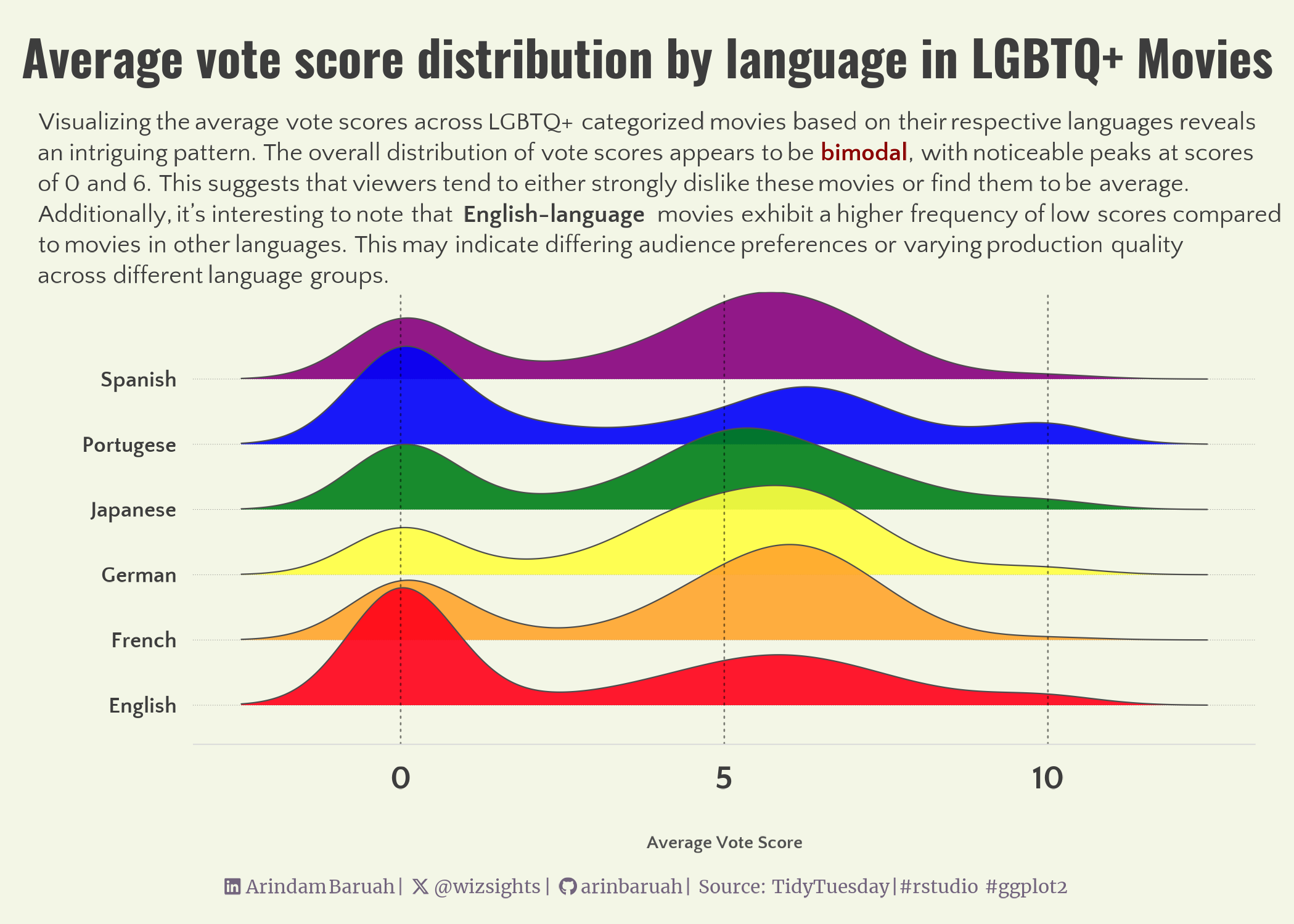
Figure 1 illustrates the average vote scores of all the LGBTQ+ categorised movies across different languages. For the current analysis, languages containing at least 100 or greater number of movies were considered.
So what do we learn from this ? 🤔🕵🏻♀️
tidyverse: Wickham H, Averick M, Bryan J, Chang W, McGowan LD, François R, Grolemund G, Hayes A, Henry L, Hester J, Kuhn M, Pedersen TL, Miller E, Bache SM, Müller K, Ooms J, Robinson D, Seidel DP, Spinu V, Takahashi K, Vaughan D, Wilke C, Woo K, Yutani H (2019). “Welcome to the tidyverse.” Journal of Open Source Software, 4(43), 1686. doi:10.21105/joss.01686 https://doi.org/10.21105/joss.01686.
glue: Hester J, Bryan J (2024). glue: Interpreted String Literals. R package version 1.7.0, https://CRAN.R-project.org/package=glue.
ggrepel: Slowikowski K (2024). ggrepel: Automatically Position Non-Overlapping Text Labels with ‘ggplot2’. R package version 0.9.5, https://CRAN.R-project.org/package=ggrepel.
ggplot2: H. Wickham. ggplot2: Elegant Graphics for Data Analysis. Springer-Verlag New York, 2016.
ggtext: Wilke C, Wiernik B (2022). ggtext: Improved Text Rendering Support for ‘ggplot2’. R package version 0.1.2, https://CRAN.R-project.org/package=ggtext.
sysfonts: Qiu Y, details. aotifSfAf (2024). sysfonts: Loading Fonts into R. R package version 0.8.9, https://CRAN.R-project.org/package=sysfonts.
showtext: Qiu Y, details. aotisSfAf (2024). showtext: Using Fonts More Easily in R Graphs. R package version 0.9-7, https://CRAN.R-project.org/package=showtext.
ggridges: Wilke C (2024). ggridges: Ridgeline Plots in ‘ggplot2’. R package version 0.5.6, https://CRAN.R-project.org/package=ggridges.