1 Introduction

Chess has been one of the most famous games to have originated from the ancient civilisations. The game is said to be about 1500 years old. It is hard to ascertain who came up with the game for the first time as different versions with identical rules were being followed at different continents and civilisations.

The precursors of the game was found to originate in 550 AD at the Gupta Empire of North Western India. The game was further introduced in early day Persia from India in around 600 AD. The game was well documented through various manuscripts as it was a marvellous game especially for those who wanted to become military commanders. It was said that chess helped build a multi approach warfare ideas. Hence, the game became extremely relevant during the times when there was no status quo amongst kingdoms and wars were frequent. At around 1850, the first Chess tournament was held in US and ever since then, it has become a sport that has been featuring in various international sports competitions like the Olympics, Commonwealth games, etc.

In this particular notebook, we will try to explore the data of women chess players and understand some key insights.

2 Importing datasets and libraries

Let us start off by importing the relevant libraries and the dataset.

Code

import numpy as np
import pandas as pd
import seaborn as sns
import matplotlib.pyplot as plt
import plotly.graph_objects as go
import plotly.express as px
from plotly.offline import download_plotlyjs, init_notebook_mode, plot, iplot

Code

df = pd.read_csv("top_women_chess_players_aug_2020.csv")
df.head()

	Fide id	Name	Federation	Gender	Year_of_birth	Title	Standard_Rating	Rapid_rating	Blitz_rating	Inactive_flag
0	700070	Polgar, Judit	HUN	F	1976.0	GM	2675	2646.0	2736.0	wi
1	8602980	Hou, Yifan	CHN	F	1994.0	GM	2658	2621.0	2601.0	NaN
2	5008123	Koneru, Humpy	IND	F	1987.0	GM	2586	2483.0	2483.0	NaN
3	4147103	Goryachkina, Aleksandra	RUS	F	1998.0	GM	2582	2502.0	2441.0	NaN
4	700088	Polgar, Susan	HUN	F	1969.0	GM	2577	NaN	NaN	wi

3 Data Cleaning

Let us check the important columns and presence of missing values if any.

First, we will try to visualise the number of missing values in each column.

Code

heatmap = sns.heatmap(df.isna(),cmap='gnuplot')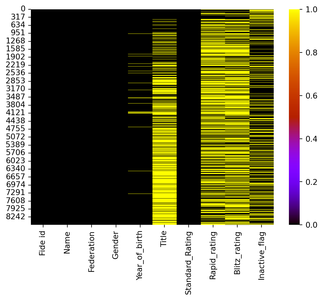

Figure 1: Missingness observed in the data

From the above figure, we can see that Year of birth, title,Rapid rating, Blitz rating and inactive_flag have a lot of null values.

Since “Fide id” and “Gender” have no purpose in our curreny analysis, we shall simply drop these columns.

Code

unn_cols=['Fide id','Gender']

for cols in unn_cols:
    df.drop(cols,axis=1,inplace=True)

Let us now check the datatypes available to us.

Code

df.dtypes

Name                object
Federation          object
Year_of_birth      float64
Title               object
Standard_Rating      int64
Rapid_rating       float64
Blitz_rating       float64
Inactive_flag       object
dtype: object

3.1 Year of birth and age

Since more than year of birth, the age of the players will be of bigger concern to us, hence we shall calculate the age of each of the players as follows. There is no way of filling the empty values here. Hence, we shall simply leave it as it is.

Code

df['Age']=2020-df['Year_of_birth']

3.2 Title

A lot of entries have null titles. This maybe assumed as new players who have not yet received an official title by FIDE which is the governing body for chess players. Hence, these null values maybe replaced by the term Unrated.

Code

df['Title']=df['Title'].fillna('Unrated')

3.3 Ratings

We see that there are null values in rapid and blitz rating. Let us fill the null values with 0 instead since it probably indicates that the player hasn’t taken part in that particular format of chess.

Code

df['Rapid_rating']=df['Rapid_rating'].fillna(0)
df['Blitz_rating']=df['Blitz_rating'].fillna(0)

3.4 Inactive flag

This flag indicates if the players are currently inactive for a fixed duration or longer. This could be for various reasons such as retirement or any other personal reasons. The null values indicate Active while WI indicates Inactive. We shall align the data into more readable form.

Code

df['Inactive_flag']=df['Inactive_flag'].fillna('Active')
df['Inactive_flag']=df['Inactive_flag'].replace('wi','Inactive')

4 Exploratory Data Analysis

Now that all our data is cleaned, we shall move ahead with the data visualisation aspect. Let’s start off with number of players from each federation.

4.1 Federation

Here, we shall visualise the top 20 most represented nations in the world.

Code

df['Count']=1
df_fed=df.groupby('Federation')['Count'].sum().reset_index().sort_values(by='Count',ascending=False)

Code

fig1=px.bar(df_fed.head(20),x='Federation',y='Count',color='Federation',labels={'Count':'Number of players'})
fig1.update_layout(template='plotly_dark',title="Top 20 most represented nations in women's Chess",title_x=0.5)
fig1.show()

Figure 2: Top 20 most represented nations in women’s Chess

From the above plot, we can see that Russia has by far the highest representation in world women’s chess followed by a distant Germany in 2nd spot. Let us try to visualise it better using a Choropleth map which will show the representation of every country.

Code

map_data = [go.Choropleth( 
           locations = df_fed['Federation'],
           locationmode = 'ISO-3',
           z = df_fed["Count"], 
           text = df_fed['Federation'],
           colorbar = {'title':'No. of Players'},
           colorscale='cividis')]

layout = dict(title = 'Players per nation', title_x=0.5,
             geo = dict(showframe = False, 
                       projection = dict(type = 'equirectangular')))

world_map = go.Figure(data=map_data, layout=layout)
iplot(world_map)

Figure 3: Top 20 most represented nations in women’s Chess

As we can see in Figure 3, Russia is very heavily represented in the Women’s world chess competition. Some key points are:

Representation from the African nations is extremely underwhelming.
Asia is well represented through India and China. Middle East Asian countries have decent representation as well. However, far East Asian countries like Thailand, Singapore, Malaysia, Vietnam and a few more are lagging behind in terms of women participation.
Oceania has relatively much lower women representation from Australia and New Zealand.
North American nations are well represented by all their countries.
Most of the South American countries are equally represented aswell.

4.2 Title

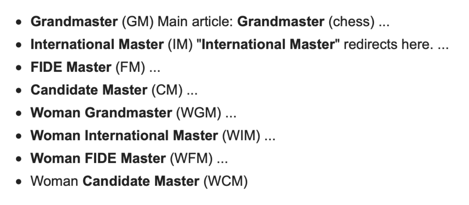
The title in Chess represents the level reached by a player. The top most position is that of a Grand Master (GM). Here is a list of all the titles that are given to players alongwith their initials.

Let us check the different titles represented by the Women through Figure 5.

Code

df_title=df.groupby('Title')['Count'].sum().reset_index().sort_values(by='Count',ascending=False)
fig2=px.pie(df_title,values='Count',names='Title',hole=0.4)
fig2.update_layout(title='Title distribution of women chess players',title_x=.5,annotations=[dict(text='Title',font_size=20, 
                                                                           showarrow=False,height=800,width=700)])
fig2.show()

Figure 5: Title distribution of women chess players

As expecred, majority of the players (about 63.5%) are still unrated. This means there are a lot of players who are yet to receive an official title from FIDE. There are only 37 women Grand masters in the world. Hence, receiving a GM title is an achievement on it’s own.

Let us now check the countries represented by the top women chess players. For considering the top chess players, we will consider the top 3 titles of GM, IM and FM

Code

df_top=df[df['Title'].isin(["GM","IM"])]

Code

fig3=px.sunburst(df_top,path=['Federation','Title'],names='Title')
fig3.update_layout(title="Title distribution per nation",title_x=0.5,template='plotly_white')
fig3.show()

Figure 6: Title distribution in each nation

Based on Figure 6, we see that China has the highest number of Grand masters with 7 followed by Russia with 6 GMs. Russia however leads the number of IMs with 15 followed by Georgia with 9 IMs.

4.3 Age

Let us check the distribution of the ages of the various chess players.

Code

fig4=px.histogram(df,x='Age',marginal='box')
fig4.update_layout(template='plotly_dark',title='Age distribution of women chess players',title_x=0.5)

Figure 7: Age distribution of the chess players

Upon checking the age distributions, we see that majority of players are within the 20-40 age group.The median age of the players is 32. Players as young as 10 year olds are also involved in competitions while the maximum age of the player till date is 100 years old.

4.4 Player activity

This indicates whether the players are currently active in chess competitions. Let us check how many players are active and how many are currently inactive.

Code

df_act=df.groupby('Inactive_flag')['Count'].sum().reset_index()
fig5=px.pie(df_act,names='Inactive_flag',values='Count',hole=0.4,color=['Purple','Red'])
fig5.update_layout(title='Activity of women Chess players',title_x=0.5,annotations=[dict(text='Activity',
                                                                                         font_size=15, showarrow=False,
                                                                                         height=800,width=700)])
fig5.update_traces(textfont_size=15,textinfo='percent+label')

fig5.show()

Figure 8: Distribution of active Chess players

From the given database, we have only about 31.6% active chess players while majority have retired or haven’t participated due to personal reasons.

4.5 Top ratings

Let us visualise the given 3 ratings of the players using a 3D scatter plot. Let us also find the average rating of each player which will indicate who has a balance of all 3 ratings. For our analysis, we shall only consider players who are currently active in chess competitions.

Code

df_a=df[df['Inactive_flag']=='Active']
df_a['Average_rating']=np.round((df_a.iloc[:,4] + df_a.iloc[:,5] + df_a.iloc[:,6])/3,2)

Code

fig6=px.scatter_3d(df_a,x='Standard_Rating',y='Blitz_rating',z='Rapid_rating',
                   color='Average_rating',size='Average_rating',opacity=1,hover_data=['Name','Standard_Rating','Blitz_rating','Rapid_rating','Average_rating'])
fig6.update_layout(margin=dict(l=0, r=0, b=0.5, t=0),title='Active player rating distributions',title_x=0.5,title_y=1)
fig6.update_traces(hovertext='Name')

fig6.show()

Figure 9: Rating distribution for each Chess player

From the 3D scatter plot illustrated by Figure 9, we can observe that Yifan Hou is the perfect player with the highest average rating of all the active players.

4.6 Radar plot of top GM, IM and FM by average ratings

In the following plot, we will see how the ratings data of each of the active top GM,IM and FM players change.

Code

df_topGM=df_a.sort_values(by='Average_rating',ascending=False).head(1)
df_topIM=df_a[df_a['Title']=='IM'].sort_values(by='Average_rating',ascending=False).head(1)
df_topFM=df_a[df_a['Title']=='FM'].sort_values(by='Average_rating',ascending=False).head(1)

cats=['Standard rating','Rapid rating','Blitz rating','Average rating']
fig7=go.Figure()
fig7.add_trace(go.Scatterpolar(r=[df_topGM.iloc[0,4],df_topGM.iloc[0,5],df_topGM.iloc[0,6],df_topGM.iloc[0,-1]],
                              theta=cats,fill='toself',name=df_topGM['Name'].values[0]+','+df_topGM['Title'].values[0]))


fig7.add_trace(go.Scatterpolar(r=[df_topIM.iloc[0,4],df_topIM.iloc[0,5],df_topIM.iloc[0,6],df_topIM.iloc[0,-1]],
                              theta=cats,fill='toself',name=df_topIM['Name'].values[0]+','+df_topIM['Title'].values[0]))

fig7.add_trace(go.Scatterpolar(r=[df_topFM.iloc[0,4],df_topFM.iloc[0,5],df_topFM.iloc[0,6],df_topFM.iloc[0,-1]],
                              theta=cats,fill='toself',name=df_topFM['Name'].values[0]+ ','+ df_topFM['Title'].values[0]))

fig7.update_layout(title='Radar plot of ratings of top GM,IM and FM',title_x=0.45)
fig7.show()

Figure 10: Rating comparison for players in various title categories

From the radar plot shown above, we see what are the differences between the top most rated GM, IM and FM.